RESULTS
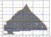
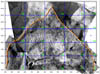
Figure 1
Figure 2
Figure 3
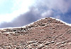
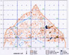
Figure 4
Figure 5
Figure 6
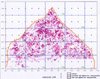
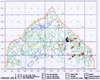
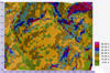
Figure 7
Figure 8
Figure 9
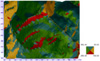
Figure 10
The data sets required for the scheme of research under the terms of the AFP-99 grant were
collected by the Kerkenes Survey Project between 1993 and 1999. These data sets were
mostly generated from the Aerial Photography, GPS Survey, Geophysical Survey and
Ground-truthing, as described below:
• Aerial Photography.
Photographs taken from aircraft, balloons and kites were studied.
The most appropriate photographs were selected for rectification
so as to permit the digitisation of visible features into a GIS
database (Fig.
3).
• GPS Survey. Some 1,250,000 readings
obtained by kinematic survey provide 80% coverage of the site.
GPS survey generates detailed simulations of the surface topography
(Fig. 1).
Geophysical Survey. A GEOSCAN Fluxgate
Gradiometer was used to collect magnetic data that reveals sub-surface
features. Processed data reveals architectural features (Fig.
2) that can then be mapped in two dimensions (Fig.
7).
• Ground-Truthing. Interpretation
of aerial photographs and geomagnetic imaging are checked against
features visible in the field. Supplementary results are then
added to the database (Fig.
6).
Some of the data was partially processed in the field, but much
further processing was undertaken at METU. More comprehensive and refined processing of
the data sets has been completed, leading to the production of working maps (Figs 1 -10).
The GPS data was converted into a very detailed terrain model using SURFER software. From
this GPS terrain model it is possible to identify and plot major features that are extant
on the surface. The geophysical maps produced in the summer of 1995, 1998 and 1999 were
then combined with the three-dimensional surface simulations.
All raw and processed data sets (rectified balloon and blimp photographs,
reconstructed defensive walls, contour maps drawn from stereo pairs
of aerial photographs, hydrology maps, geological fault maps, etc.)
have been transferred into Intergraph Systems software, which permits
comparative display of the different elements. The accuracy of values
calculated for the different data sets are within acceptable limits,
as can be seen in the combined images (e.g.
Fig. 4).
During the transfer of data sets into GIS, local site co-ordinates
were converted to the UTM (Universal Transverse Mercator) co-ordinate system. This
conversion increases the scope for future data intake as well as enabling certain elements
of the GIS software to function with greater efficiency. The GIS also allows simultaneous
display of the local co-ordinate system that is used for data collection in the field. The
local site grid is sub-divided into 200 x 300m rectangles from an arbitrary 0.0 point.
Each grid rectangle is designated by a label that is alphabetical along the x axis and
numerical along the y axis (e.g. A1). This simple system was designed for ease of
reference and printing on standard A-size paper. Sub-division into 100 x 100m grid squares
is followed by further division into a 20 x 20m grid system for geophysical survey. Any
grid or reference point is located according to its unique co-ordinate (e.g. grid
e220n140).
Two-dimensional geophysical survey images were also transposed onto
very detailed GPS three-dimensional terrain models (Fig.
5). In an earlier study, geophysical imagery was overlaid on
the 5m interval contour map in ways that enhanced visibility
of the close spatial relationships between certain elements of the
urban infrastructure, including: topography and the line of the
city defences, hydrology and the positioning of elements within
the elaborate system of water management, the network of urban communications
and the planned layout of urban blocks, the positioning of public
space and monumental architecture. In short, we were beginning to
recognise the dynamics of urban zoning. In this latest, more detailed,
study it has been possible to ascertain which walls can be seen
both on the geophysical (sub-surface) images and on the GPS (surface)
model. These results will be invaluable in the application of higher
levels of GIS analyses (e.g. slope aspect and view shed). Because
of the magnitude of the GPS data the mapping has been done in 18
separate areas that have then been combined into a single map.
Ground-truthing studies have been assessed, finalised and then digitised
into the GIS database (Fig.
6). Categories of recorded surface features that were selected
for insertion into the GIS database as separate layers comprised:
bedrock, vegetation, Iron Age walls, probable Iron Age walls, modern
enclosures, tumuli, wet areas (at the time recorded) and water courses.
Data and image processing of the geophysical survey was also finalised
during the post-fieldwork period and the results digitised into
the GIS media (Fig.
7). Walls were classified into two categories: “certain Iron
Age” and “probable Iron Age”.
From the digitised data sets, the main architectural features (urban
blocks, reservoirs, etc) of the northern portion of the site were
plotted and displayed together with other relevant data (Fig.
8). Definable patterns related to communications, habitations,
water resources, etc., emerge from these maps. These patterns can
be compared with maps generated from physical and environmental
data, e.g. slope and aspect maps (Figs
9 and 10),
that may indicate how the choice of certain areas for specific functions
might be related to the physical characteristics of the terrain,
slope orientation or other environmental issues. In this way, such
cultural considerations as might have influenced the city planning
can be highlighted.
In the next stage of analyses, a typological classification will be imposed on the
features according to predetermined sets of criteria. Each class of features will be
entered as a separate layer within the GIS environment. The features will then be
classified according to what they are understood to represent (building, type of building,
vegetation, bedrock, burnt debris, etc.). Some types of these classes may then be
subdivided into sub-classes (e.g. walls, doors, and pavements). Due to the archaeological
nature of the material which, of necessity, has to be subjected to a considerable degree
of interpretation, the classification will be flexible during this initial stage. The
approach will entail GIS driven spatial analysis of known features (e.g. streets and urban
blocks), followed by inclusion of those classes of data that require a higher degree of
interpretation in order for a scheme of classification to be imposed upon them.